Simulations#
The atooms’ interface abstracts out most of the common tasks of particle-based simulations. The actual simulation is performed by a simulation “backend”, which exposes a minimal but consistent interface. This enables one to develop complex simulation frameworks (e.g., parallel tempering) that are essentially decoupled from the underlying simulation code.
A Simulation is a high-level class that encapsulates some common tasks, like regularly storing data on files, and provides a consistent interface to the user, while backend classes actually make the system evolve. Here, we implement a minimal backend to run a simulation.
At a very minimum, a backend is a class that provides
a system instance variable, which should (mostly) behave like
atooms.system.Systema run() method, which evolves the system for a prescribed number of steps (passed as argument)
Optionally, the backend may hold a reference to a trajectory class, which can be used to checkpoint the simulation or to write configurations to a file. This is however not required in a first stage.
A minimal simulation backend#
We set up a bare-bones simulation backend building on the native System class
from atooms.system import System

class BareBonesBackend(object):

    def __init__(self):
        self.system = System()

    def run(self, steps):
        for i in range(steps):
            pass

# The backend is created and wrapped by a simulation object.
# Here we first call the run() method then run_until()
from atooms.simulation import Simulation
from atooms.simulation.core import _log as logger
backend = BareBonesBackend()
simulation = Simulation(backend)
simulation.run(10)
simulation.run_until(30)
assert simulation.current_step == 30

# This time we call run() multiple times
simulation = Simulation(backend)
simulation.run(10)
simulation.run(20)
assert simulation.current_step == 30

# Set up verbose logging to see a meaningful log
from atooms.core.utils import setup_logging
setup_logging(level=20, update=True)
simulation = Simulation(backend)
simulation.run(10)
setup_logging(level=40, update=True)
#
# atooms simulation via <__main__.BareBonesBackend object at 0x7f6f4f8e1430>
#
# version: 3.14.1+3.14.1-7-g7ec3c6-dirty (2022-12-10)
# atooms version: 3.14.1+3.14.1-7-g7ec3c6-dirty (2022-12-10)
# simulation started on: 2022-12-21 at 11:04
# output path: None
# backend: <class '__main__.BareBonesBackend'>
#
# target target_steps: 10
#
#
# <__main__.BareBonesBackend object at 0x7f6f4f8e1430>
# simulation ended successfully: reached target steps 10
#
# final steps: 10
# final rmsd: 0.00
# wall time [s]: 0.00
# average TSP [s/step/particle]: nan
# simulation ended on: 2022-12-21 at 11:04
Simple random walk#
We implement a simple random walk in 3d. This requires adding code to the backend run() method to actually move the particles around. The code won’t be very fast! See below Faster backends.
We start by building an empty system. Then we add a few particles and place them at random in a cube. Finally, we write a backend that displaces each particle randomly over a cube of prescribed side.
import numpy
from random import random
from atooms.system import System
from atooms.system.particle import Particle

system = System()
L = 10
for i in range(1000):
    p = Particle(position=[L * random(), L * random(), L * random()])
    system.particle.append(p)

class RandomWalk(object):

    def __init__(self, system, delta=1.0):
        self.system = system
        self.delta = delta

    def run(self, steps):
        for i in range(steps):
            for p in self.system.particle:
                dr = numpy.array([random()-0.5, random()-0.5, random()-0.5])
                dr *= self.delta
                p.position += dr
Adding callbacks#
The Simulation class allows you to execute of arbitrary code during the simulation via “callbacks”. They can be used for instance to
store simulation data
write logs or particle configurations to trajectory files
perform on-the-fly calculations of the system properties
define custom conditions to stop the simulation
Callbacks are plain function that accept the simulation object as first argument. They are called at prescribed intervals during the simulation.
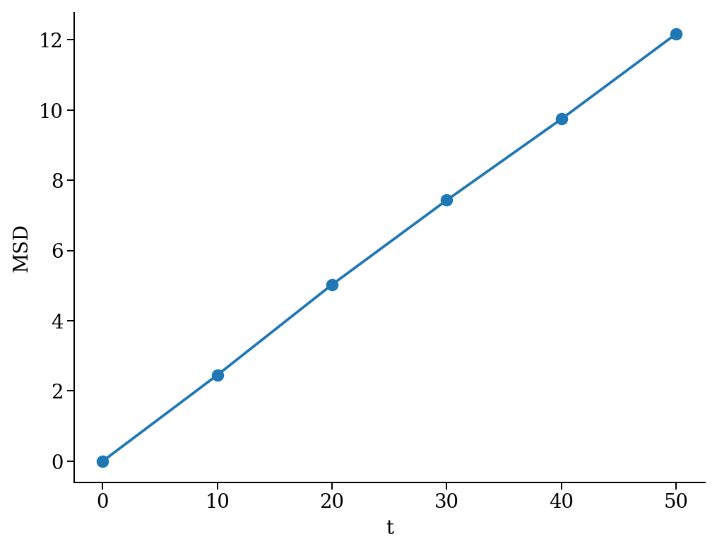
As an example, we measure the mean square displacement (MSD) of the particles to make sure that the system displays a regular diffusive behavior \(MSD \sim t\)
from atooms.simulation import Simulation
simulation = Simulation(RandomWalk(system))

# We add a callback that computes the MSD every 10 steps
# We store the result in a dictionary passed to the callback
msd_db = {}
def cbk(sim, initial_position, db):
    msd = 0.0
    for i, p in enumerate(sim.system.particle):
        dr = p.position - initial_position[i]
        msd += numpy.sum(dr**2)
    msd /= len(sim.system.particle)
    db[sim.current_step] = msd

# We will execute the callback every 10 steps
simulation.add(cbk, 10, initial_position=[p.position.copy() for p in
                                          system.particle], db=msd_db)
simulation.run(50)

# The MSD should increase linearly with time
time = sorted(msd_db.keys())
msd = [msd_db[t] for t in time]
The MSD as a function of time should look linear.
import matplotlib.pyplot as plt
plt.plot(time, msd, '-o')
plt.xlabel("t")
plt.ylabel("MSD")
The postprocessing component package provides way more options to compute dynamic correlation functions.
Fine-tuning the scheduler#
Calling a callback can be done at regular intervals during the simulation or according to a custom schedule defined by a Scheduler. Here we consider the simulation.write_trajectory() callback, which writes the system state in a trajectory file
from atooms.trajectory import TrajectoryXYZ
from atooms.simulation import write_trajectory, Scheduler

simulation = Simulation(RandomWalk(system))
trajectory = TrajectoryXYZ('/tmp/trajectory.xyz', 'w')
# Write every 10 steps
simulation.add(write_trajectory, Scheduler(10), trajectory=trajectory)
Here are a few options of the Scheduler:
interval: notify at a fixed steps interval (default)calls: fixed number of calls to the callbacksteps: list of steps at which the callback will be calledblock: as steps, but the callback will be called periodicallyseconds: notify everyseconds
One useful application of the Scheduler is writing frames in a trajectory at exponentialy spaced intervals. Here the
trajectory_exp = TrajectoryXYZ('/tmp/trajectory_exp.xyz', 'w')
simulation.add(write_trajectory, Scheduler(block=[0, 1, 2, 4, 8, 16]), trajectory=trajectory_exp)
simulation.run(32)
trajectory.close()
trajectory_exp.close()
Now we will have two trajectories, one with regular and the other with exponentially spaced blocks of frames
with TrajectoryXYZ('/tmp/trajectory.xyz') as th, \
     TrajectoryXYZ('/tmp/trajectory_exp.xyz') as th_exp:
    print('Regular:', th.steps)
    print('Exponential:', th_exp.steps)
Regular: [0, 10, 20, 30]
Exponential: [0, 1, 2, 4, 8, 16, 17, 18, 20, 24, 32]
Compute statistical averages#
The simulation.store() callback allows you to store data in a dictionary while the simulation is running. Here are a few ways to use it to perform some statistical analysis.
The store callback accepts an array of arguments to store. They can be string matching a few predefined attributes (such as steps, the current number of steps carried out by the backend) or a general attribute of the simulation instance (such as system.particle[0].position[0], the x-coordinate of the first particle of the system).
import numpy
from atooms.simulation import store

simulation = Simulation(RandomWalk(system))
simulation.add(store, 1, ['steps', 'system.particle[0].position[0]'])
By default, after running the simulation, the data will be stored in the simulation.data dictionary and you can use it for further analysis
import numpy
simulation.run(10)
print(numpy.mean(simulation.data['system.particle[0].position[0]']))
2.493414801026613
You can store the result of any function that takes as first argument the simulation instance. Just add a tuple with a label and the function to the list of properties to store.
simulation = Simulation(RandomWalk(system))
simulation.add(store, 1, ['steps', ('x_1', lambda sim: sim.system.particle[1].position[0])])
simulation.run(10)
Faster backends#
Moving particles using the Particle object interface is expressive but computationally very slow, since it forces us to operate one particle at a time. We can write a more efficient backend by getting a “view” of the system’s coordinates as a numpy array and operating on it vectorially. You can also pass the viewed arrays to backends written in compiled languages (even just in time).
import numpy
from atooms.system import System

# Create a system with 10 particles
system = System(N=10)

class FastRandomWalk(object):

    def __init__(self, system, delta=1.0):
        self.system = system
        self.delta = delta

    def run(self, steps):
        # Get a view on the particles' position
        pos = self.system.view("position")
        for i in range(steps):
            dr = (numpy.random(pos.shape) - 0.5) * self.delta
            # Operate on array in-place
            pos += dr
Note
Here is the recommended approach:
get a view of the arrays you need once at the beginning of
run()if possible, operate on those arrays in-place
if you make copies of the arrays, update the viewed arrays at the end of
run()
This way the attributes of the Particle objects will remain in sync with viewed arrays
The viewed array can be cast in C-order (default) or F-order using the order parameter
system.view("position", order='C')
system.view("position", order='F')
If \(N\) is the number of particles and \(d\) is the number of spatial dimensions, then you’ll get
$(N, d)$-dimensional arrays with
order’C’= (default)$(d, N)$-dimensional arrays with
order’F’=
Of course, this option is relevant only for vector attributes like positions and velocities.
You can get a view of any system property by providing a “fully qualified” attribute
assert numpy.all(system.view("cell.side") == system.cell.side)
In particular, for particles’ attributes you can use this syntax
assert numpy.all(system.view("particle.position") == system.view("pos"))
Molecular dynamics with LAMMPS#
Atooms provides a simulation backend for LAMMPS, an efficient and feature-rich molecular dynamics simulation package.
The backend accepts a string variable containing regular LAMMPS commands and initial configuration to start the simulation. The latter can be provided in any of the following forms:
a
Systemobjecta
Trajectoryobjectthe path to an xyz trajectory
In the last two cases, the last configuration will be used to start the simulation.
Here we we use the first configuration of an existing trajectory for a Lennard-Jones fluid
import os
from atooms.core.utils import download
import atooms.trajectory as trj
from atooms.backends import lammps

# You can change it so that it points to the LAMMPS executable
lammps.lammps_command = 'lmp'

download('https://framagit.org/atooms/atooms/raw/master/data/lj_N1000_rho1.0.xyz', "/tmp")
system = trj.TrajectoryXYZ('/tmp/lj_N1000_rho1.0.xyz')[0]
cmd = """
pair_style      lj/cut 2.5
pair_coeff      1 1 1.0 1.0  2.5
neighbor        0.3 bin
neigh_modify    check yes
timestep        0.002
"""
backend = lammps.LAMMPS(system, cmd)
We now wrap the backend in a simulation instance. This way we can rely on atooms to write thermodynamic data and configurations to disk during the simulation: we just add the write_config() and write_thermo() callbacks to the simulation.
You can add your own functions as callbacks to perform arbitrary manipulations on the system during the simulation. Keep in mind that calling these functions causes some overhead, so avoid calling them at too short intervals.
from atooms.simulation import Simulation
from atooms.system import Thermostat
from atooms.simulation.observers import store, write_config

# We create the simulation instance and set the output path
sim = Simulation(backend, output_path='/tmp/lammps.xyz')
# Write configurations every 1000 steps in xyz format
sim.add(write_config, 1000, trajectory_class=trj.TrajectoryXYZ)
# Store thermodynamic properties every 500 steps
sim.add(store, 100, ['steps', 'potential energy per particle', 'temperature'])
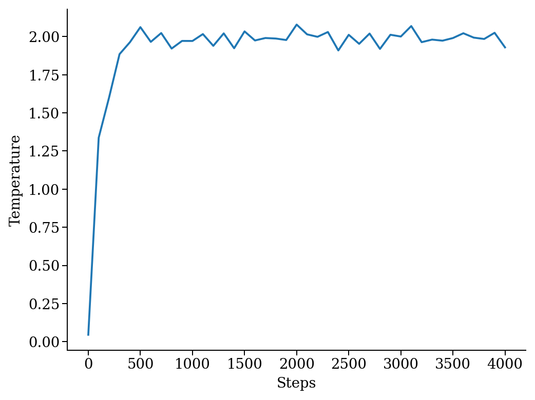
We add a thermostat to keep the system temperature at T=2.0 and run the simulations for 10000 steps.
backend.system.thermostat = Thermostat(temperature=2.0, relaxation_time=0.1)
sim.run(4000)
Note that we use atooms Thermostat object here: the backend will take care of adding appropriate commands to the LAMMPS script.
We have a quick look at the kinetic temperature as function of time to make sure the thermostat is working
plt.plot(sim.data['steps'], sim.data['temperature'])
plt.xlabel('Steps')
plt.ylabel('Temperature')
We can then use the postprocessing package to compute the radial distribution function or any other correlation function from the trajectory.
Molecular dynamics with RUMD#
There is native support for an efficient MD molecular dynamics code running entirely on GPU called RUMD, developed by the Glass and Time group in Roskilde. It is optimized for small and medium-size systems.
Here we pick the last frame of the trajectory, change the density of the system to unity and write this new configuration to a trajectory format suitable for RUMD
from atooms.trajectory import Trajectory

with Trajectory('/tmp/lj_N1000_rho1.0.xyz') as trajectory:
    system = trajectory[-1]
    system.density = 1.0
    print('New density:', round(len(system.particle) / system.cell.volume, 2))

from atooms.trajectory import TrajectoryRUMD
with TrajectoryRUMD('rescaled.xyz.gz', 'w') as trajectory:
    trajectory.write(system)
New density: 1.0
Now we run a short molecular dynamics simulation with the RUMD backend, using a Lennard-Jones potential:
import rumd
from atooms.backends.rumd import RUMD
from atooms.simulation import Simulation

potential = rumd.Pot_LJ_12_6(cutoff_method=rumd.ShiftedPotential)
potential.SetParams(i=0, j=0, Epsilon=1.0, Sigma=1.0, Rcut=2.5)
backend = RUMD('rescaled.xyz.gz', [potential], integrator='nve'
sim = Simulation(backend)
sim.run(1000)
A repository of interaction models for simple liquids and glasses is available in the atooms-models component package. It generates RUMD potentials automatically from standardized json file or Python dictionaries.